Racing Line Optimization Maps the Fastest Track Trajectory

Imagine the perfect lap – every corner apex hit precisely, every straight maximized for speed, a dance between machine and asphalt that shaves milliseconds off the clock. This isn't just a fantasy for professional drivers; it's a solvable engineering problem. Racing Line Optimization is the sophisticated process of mathematically determining the absolute fastest, safest, and most efficient path around any given racetrack. For autonomous vehicles like the F1TENTH or even in professional motorsport simulations, it’s the secret sauce that transforms a raw track map into a high-performance trajectory.
This isn't about guesswork; it's about leveraging advanced algorithms to unlock a track's true speed potential. From the intricate turns of Monaco to the sweeping curves of Spa-Francorchamps, optimizing the racing line provides a definitive, data-driven strategy.

At a Glance: What You'll Learn

What it is: The process of mathematically finding the optimal path for a vehicle around a track.
Why it matters: Maximizes average speed, ensures safety, and provides a precise driving trajectory for autonomous systems or human training.
The core steps: How a raw map evolves into a high-fidelity racing line.
Key optimization strategies: Understanding minimum time versus other approaches.
Critical parameters: How friction, safety margins, and computational speed impact the outcome.
Hands-on application: A practical guide to implementing racing line optimization using open-source tools.
Troubleshooting: Solutions to common setup and execution issues.

The Quest for the Perfect Path: Why Optimize?

Every racer knows the adage: "Slow in, fast out." But what does "slow" really mean? And where exactly is "out"? For human drivers, years of experience, instinct, and a feel for the car guide these decisions. For autonomous systems, or for engineers striving to push the limits of performance, that intuition needs to be codified into hard data. This is where Racing Line Optimization steps in.
The goal isn't merely to find the shortest path, which might involve sharp, slow corners. Instead, it's to find the path that allows the vehicle to maintain the highest average speed, considering its dynamic capabilities (acceleration, braking, grip limits) and the track geometry. This intricate balance is why optimization is crucial for projects like the F1TENTH, where every millisecond counts in high-speed, autonomous racing.

From Blank Canvas to Blistering Speed: The Optimization Journey

Generating an optimal racing line is a multi-stage process that systematically builds from a basic track layout to a detailed, high-speed trajectory. Think of it as sculpting a masterpiece, one precise step at a time.

Step 1: Charting the Terrain – Map Generation

Before you can race, you need a track. The first hurdle is translating the physical world into a digital representation. This typically begins with creating an Occupancy Grid map, often using tools like slam_toolbox. This process effectively scans the environment and categorizes every pixel:

Occupied (Black): Represents walls, barriers, or other impassable obstacles.
Free (White): Designates the open, drivable area.
Unknown (Gray): Areas the sensor hasn't yet observed.
The output of this mapping phase is usually a .pgm file (a grayscale image of the track) and a .yaml file. The .yaml file is essential; it contains metadata like the map's origin and resolution, allowing the system to accurately convert image pixels into real-world coordinates (like meters). This fundamental step ensures the digital model is an accurate reflection of the physical track.

Step 2: Refining the Blueprint – Map Editing

Raw sensor data rarely provides a perfect, race-ready track. Maps generated by SLAM tools often have open sections or irregularities that aren't ideal for trajectory planning. This is where manual refinement comes in. You'll typically use image editing software, such as Photoshop, to "close" the racetrack.
The objective here is to clearly define the boundaries of the drivable area, transforming an ambiguous sensor map into a clean, closed circuit. For very large maps, you might only need to draw the white, drivable area; specialized scripts can then infer and generate the necessary edges. This step is critical because a well-defined track boundary is paramount for subsequent centerline generation and precise optimization.

Step 3: Finding the Middle Ground – Centerline and Track Widths

With a clean, closed map, the next step is to extract the track's fundamental geometry: its centerline and width at every point. The raceline optimizer doesn't just need a picture of the track; it needs a structured data representation.
This involves identifying a series of (x,y) coordinates that define the track's centerline. For each of these points, you also need to specify wl (the distance to the left boundary) and wr (the distance to the right boundary). These measurements are crucial as they define the 'wiggle room' the vehicle has at any given segment of the track. Once these points are defined, they are smoothly connected using a cubic Spline, creating a continuous, differentiable centerline that the optimization algorithm can work with. This precise geometric data allows the optimizer to understand the track's constraints and opportunities in detail.

Step 4: Unleashing the Algorithms – Running the Optimization

This is the core of Racing Line Optimization. With a detailed centerline and track width information, an advanced optimization algorithm takes over. Its mission: to adjust the reference line (the centerline) to maximize the vehicle's average speed around the track, all while strictly adhering to the physical limitations of the vehicle (e.g., maximum cornering force, acceleration, braking) and the boundaries of the track.
This is an iterative process. The algorithm makes small adjustments to the path, simulates the vehicle's performance, and then refines the path again, repeating until no further significant improvements can be made – a state known as convergence.
Steven Gong's widely recognized implementation, for instance, often employs a mintime (minimum time) approach. This is generally the most performance-oriented objective, though it's also the most computationally intensive. Other formalizations include:

Shortest Possible Path: Prioritizes minimal distance, often resulting in sharp, sub-optimal turns for speed.
Minimum Curvature: Aims for the smoothest possible path, reducing lateral G-forces and improving stability, which indirectly contributes to speed but might not be the absolute fastest.
Minimum Time: The gold standard for racing, directly optimizing for the lowest possible lap time. This approach factors in vehicle dynamics like acceleration, braking, and tire grip, making it significantly more complex but yielding the most realistic high-performance trajectory.
The final racing line is typically exported as a .csv file. Each row in this file contains a (x, y, v) tuple, providing a precise target (x,y) position and the optimal velocity v the vehicle should aim for at that specific point on the track.

Fine-Tuning Your Trajectory: Key Parameters

The effectiveness of your racing line optimization heavily relies on accurately configuring a few critical parameters. These settings essentially tell the algorithm about the vehicle's capabilities and the track's characteristics. You'll often find these adjustable in configuration files like f110.ini or similar parameter files.

Friction (mu or similar): This is arguably the most crucial parameter, representing the coefficient of friction between the tires and the track surface. It directly dictates the maximum grip available for cornering, acceleration, and braking. An accurate friction value is vital for a realistic racing line. Values vary significantly:
Asphalt: 0.6 - 0.9
Concrete: 0.5 - 0.8
Rubberized tracks (e.g., some indoor kart tracks): 0.9 - 1.1 (due to high grip compounds)
Gravel: 0.4 - 0.8
Grass: 0.2 - 0.4
Sand: 0.1 - 0.3
For a slippery track, you might use a value like 0.4 to generate a more conservative line.
Safety Margin (width_opt): This parameter allows you to control how close the optimized racing line gets to the track boundaries (walls). A larger safety margin means the vehicle will stay further from the edges, increasing safety but potentially sacrificing a little speed. A smaller margin pushes the line closer to the limits, maximizing track utilization but increasing risk. It’s a trade-off between aggression and caution.
Optimization Speed (step sizes): If the optimization process is taking too long to converge, you can often adjust parameters related to the algorithm's step size or iteration count. Increasing step sizes can make the optimization faster by taking larger jumps between iterations, but it might also reduce precision or risk missing the absolute optimal solution. Conversely, smaller steps increase accuracy but prolong computation.

From Concept to Code: Implementing Racing Line Optimization

Many researchers and enthusiasts leverage open-source repositories to implement racing line optimization. The Raceline-Optimization repository, for instance, provides a robust framework for determining optimal lines with various objectives. Let's walk through how you might use such a system.

Repository Components at a Glance

A typical racing line optimization repository is structured to manage various aspects of the process:

frictionmap: Dedicated functions for generating and handling track-specific friction maps.
helper_funcs_glob: A collection of utility functions aiding in global trajectory calculations.
inputs: Where you'll store vehicle dynamics profiles, reference track CSVs, and custom friction maps.
opt_mintime_traj: Contains the core algorithms for time-optimal trajectory generation, including considerations for powertrain behavior via powertrain_src.
params: Configuration files for optimization settings and vehicle-specific parameters.

Getting Started and Running the Code

Clone and Setup: Begin by cloning the repository to your local machine. It's highly recommended to set up a virtual environment (Conda is an excellent choice) to manage dependencies cleanly.
Install Dependencies: Install all required Python packages. Be aware that some specific versions or forks might be needed. For example, a fork of trajectory planning helpers might be used to resolve common issues with the quadprog library.
Map Preparation: This is crucial for defining your racetrack.

SLAM-generated maps: If you're starting with an Occupancy Grid map from slam_toolbox, you'll first run a map_converter.ipynb script, followed by sanity_check.ipynb. This process takes your .pgm and .yaml files and exports a .csv map into the inputs/tracks directory, making it readable for the optimizer.
Waypoint-generated maps: If you already have a track defined by a series of waypoints, you can typically store this .csv file directly in inputs/tracks.

Execute Trajectory Generation: The main script, often named main_globaltraj_f110.py (or similar), is your gateway to generating the racing line. You'll run this script, typically specifying the map name as an argument:
bash
python main_globaltraj_f110.py --map_name your_track_name
By default, the generated raceline will be saved in an outputs/<map_name> directory. You can often specify custom output paths using --map_path and --export_path arguments.

Configuration Steps for Execution

Before running the main script, you might want to tailor the optimization to your specific needs:

Parameter Adjustment (Optional): Dive into the params folder to fine-tune various optimization and vehicle settings. This is where you adjust friction, safety margins, and other core parameters.
Vehicle Dynamics (Optional): For precise acceleration calculations without considering drag, you can modify the ggv diagram and ax_max_machines in inputs/veh_dyn_info. This allows you to model your vehicle's performance characteristics accurately.
Custom Tracks and Friction Maps (Optional): If you've prepared your own reference track files, place them in inputs/tracks. Similarly, custom friction map files go into inputs/frictionmaps.
Powertrain Behavior (Optional): To introduce a more sophisticated model that considers the vehicle's powertrain:
Enable the powertrain option in your parameter file.
Adjust the number of laps in the main_globaltraj.py script.
Decide between simple_loss = True (an approximation) or False (detailed models) in params/racecar.ini for power loss calculations.
Final Script Adjustments: Make any last-minute parameter tweaks directly within the main_globaltraj.py script itself, then execute it. The resulting optimized trajectory will be saved, typically as outputs/traj_race_cl.csv.

Common Roadblocks & How to Overcome Them

Working with advanced optimization libraries can sometimes lead to installation headaches. Here are a few common issues and their solutions:

Windows cvxpy and quadprog issues: These libraries often require a C++ compiler.
Solution: Download and install the Visual Studio 2019 build tools (specifically the "C++ build tools" option). This provides the necessary compiler for Python packages. For quadprog itself, trying a specific version like 0.1.6 can often resolve compatibility problems.
Ubuntu matplotlib and tkinter: matplotlib, a popular plotting library, sometimes requires the tkinter backend for full functionality, especially when running interactively.
Solution: Run sudo apt install python3-tk to install the tkinter development files.
Ubuntu Python.h needed by quadprog: When installing quadprog or similar C-extension Python packages, you might encounter an error indicating that Python.h is missing.
Solution: Install the Python development headers by running sudo apt install python3-dev.

Beyond the Basics: Friction Maps and Powertrain Dynamics

For truly advanced Racing Line Optimization, two concepts offer significant enhancements:

Creating Friction Maps

The main_gen_frictionmap.py script allows you to generate custom friction maps. Instead of a single, uniform friction coefficient for the entire track, a friction map can define varying grip levels across different sections. Imagine a track with a patch of oil, a damp corner, or a section of older asphalt—a friction map can model these nuances. These maps are stored in inputs/frictionmaps and are particularly valuable when pursuing minimum time optimization, as they provide a more realistic model of available grip.

Powertrain Behavior Consideration

Standard minimum time optimization often assumes ideal power delivery. However, a vehicle's actual powertrain behavior (e.g., gear shifts, torque curves, engine efficiency, transmission losses) significantly impacts its real-world acceleration and top speed. By enabling powertrain consideration, the optimization algorithm can factor in these more detailed models, leading to a racing line that is not only geometrically optimal but also dynamically achievable given the vehicle's specific power unit. This level of detail results in highly realistic and implementable trajectories.

Understanding the Output: Your Optimized Trajectory Files

After the optimization algorithm has crunched the numbers, the result is a highly detailed .csv file representing your racing line. The file_paths dictionary in main_globtraj.py typically controls the output format. Two common formats offer different levels of detail:

1. Race Trajectory (Default)

This format provides a concise yet comprehensive overview of the optimized racing line, typically as an array [no_points x 7]. Each row details a specific point along the trajectory:

s_m (float32, meter): The curvilinear distance measured along the raceline from the start.
x_m (float32, meter): The X-coordinate of the raceline point in the world frame.
y_m (float32, meter): The Y-coordinate of the raceline point in the world frame.
psi_rad (float32, rad): The heading (orientation) of the raceline at this point, typically from -π to +π, with zero indicating north.
kappa_radpm (float32, rad/meter): The curvature of the raceline at this point. Higher curvature means a sharper turn.
vx_mps (float32, meter/second): The target velocity the vehicle should achieve at this point.
ax_mps2 (float32, meter/second²): The target acceleration the vehicle should maintain (often assumed constant until the next point).
This format is excellent for visualizing the trajectory, feeding into lower-level controllers, or simply understanding the optimal speed profile.

2. LTPL Trajectory

The "Local Trajectory Planner Link" (LTPL) format is more comprehensive, designed to be directly ingested by a graph-based local trajectory planner. It's an array [no_points x 12] that includes additional reference and normal vector information:

x_ref_m, y_ref_m: X and Y coordinates of the original reference line point (often the centerline).
width_right_m, width_left_m: The distances from the x_ref_m, y_ref_m point to the right and left track boundaries, respectively.
x_normvec_m, y_normvec_m: X and Y coordinates of the normalized normal vector at the reference point. (Normal vectors typically point to the right in the direction of driving).
alpha_m: The lateral shift solution from the optimization. This tells you how far the optimized raceline point has shifted laterally from the original reference line.
s_racetraj_m: Curvilinear distance along the actual optimized raceline.
psi_racetraj_rad: Heading of the optimized raceline.
kappa_racetraj_radpm: Curvature of the optimized raceline.
vx_racetraj_mps: Target velocity of the optimized raceline.
ax_racetraj_mps2: Target acceleration of the optimized raceline.
This detailed format provides all the necessary context for subsequent planning stages, allowing a local planner to generate smooth, immediate actions based on the global optimal path.

Mastering the Art and Science of the Racing Line

Racing Line Optimization isn't just for robots. By understanding the principles and outputs of these algorithms, human drivers can gain incredible insights into their own track performance. It demystifies the "art" of driving by providing a scientific basis for optimal cornering, braking points, and acceleration zones.
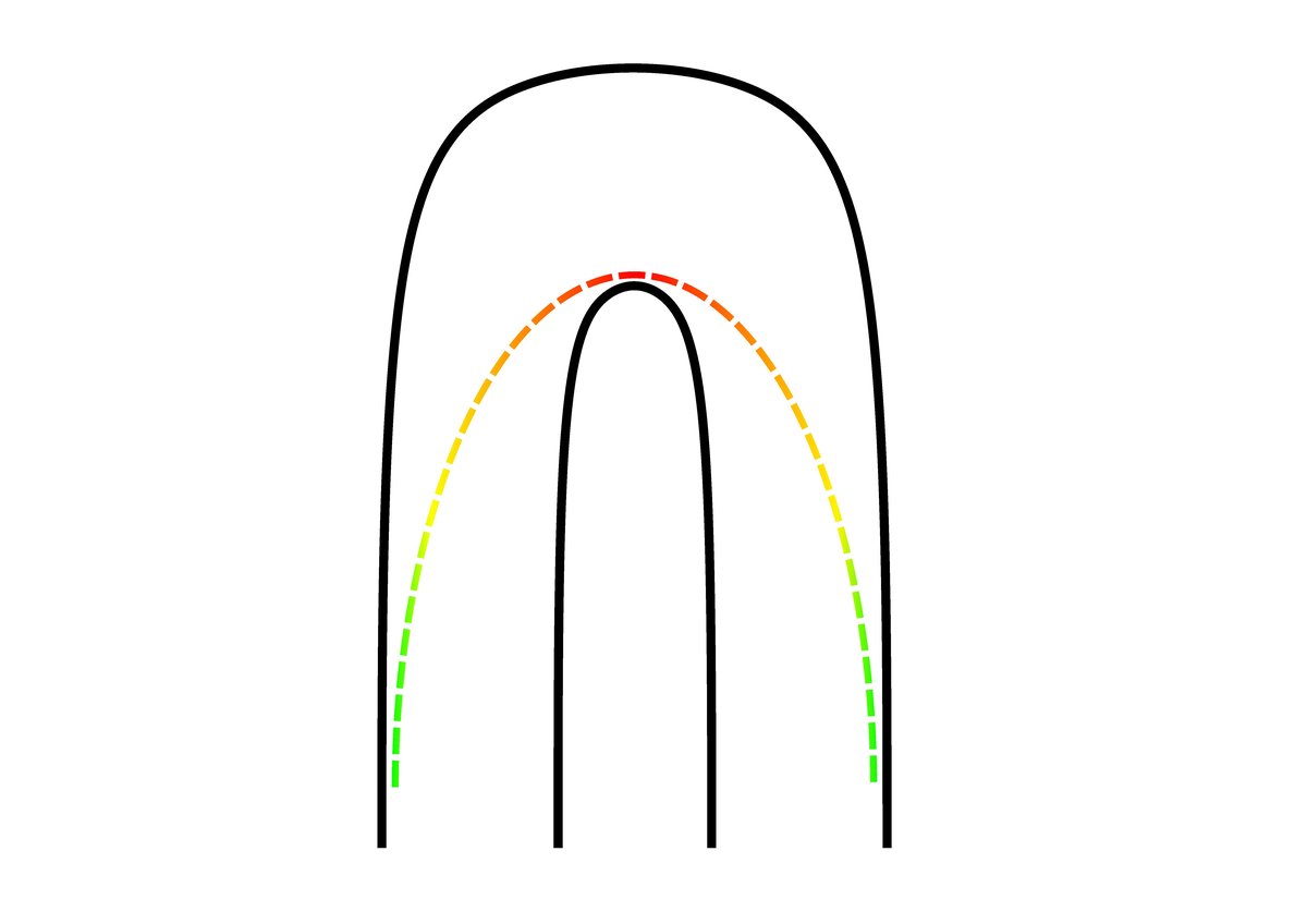
For instance, visualizing an optimized racing line often highlights the importance of using the full width of the track, particularly when entering a corner wide to open up the exit. This allows for a smoother arc and enables the driver to carry more speed through the turn, a principle known as the outside-inside-outside rule. Applying these data-driven insights can refine a driver's technique and shave precious tenths off their lap times, making the "perfect lap" less of an elusive dream and more of an attainable goal.
Whether you're building an autonomous race car, simulating performance for a professional team, or simply trying to improve your own track driving, understanding and leveraging Racing Line Optimization maps the fastest, most efficient trajectory to success. It combines the rigorous logic of mathematics with the exhilarating pursuit of speed, giving you an unparalleled advantage on any circuit.